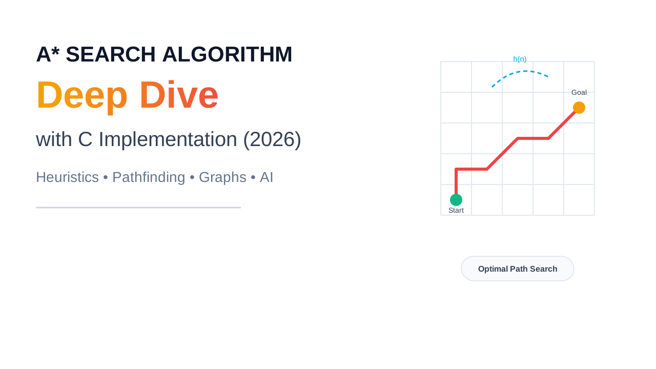
The Shortest Path to the Right Answer
In the winter of 1967, a team at Stanford Research Institute was trying to automate a mobile robot named Shakey. Shakey needed to navigate physical spaces — move around obstacles, find goals, plan routes through an environment it could see with a camera. The pathfinding algorithms of the time either explored blindly (expanding every reachable node, regardless of whether it looked promising) or relied on simple heuristics without any guarantee of finding the shortest path.
Peter Hart, Nils Nilsson, and Bertram Raphael were dissatisfied with that trade-off. They wanted an algorithm that was simultaneously fast and guaranteed-optimal. In 1968, they published “A Formal Basis for the Heuristic Determination of Minimum Cost Paths” — and introduced A* search.
Fifty-six years later, A* is the backbone of pathfinding in virtually every domain where finding the optimal route matters: video games routing NPCs and players, GPS navigation systems computing driving directions, robotics planning motion through physical space, logistics networks optimizing delivery routes, and increasingly, AI planning systems deciding the sequence of actions an agent should take to achieve a goal.
Understanding A* deeply — not just “it uses a heuristic to be smarter than Dijkstra” but the precise mathematical conditions that make it optimal, the data structure decisions that determine its performance, and the implementation details that separate a correct algorithm from a fast and correct one — is foundational knowledge for any software engineer who works on search, planning, AI, or optimization. This article builds that understanding from first principles and finishes with a complete, working C implementation.
Phase 1: The Problem — Why Smarter Search Was Necessary
The Explosion of Blind Search
The most naive approach to finding a path between two nodes in a graph is breadth-first search: start at the source node, explore all neighbors, then all neighbors-of-neighbors, expanding outward in concentric rings until you reach the destination. BFS is guaranteed to find the shortest path in an unweighted graph, and its correctness is easy to prove. Its problem is efficiency.
In a grid that is 100 × 100 cells — not large by any practical standard — there are 10,000 nodes. If the goal happens to be far away, BFS may expand thousands of nodes before reaching it, regardless of which direction the goal is in. It has no concept of “closer” or “farther” — it treats every unexplored neighbor as equally worth investigating. On a 1000 × 1000 grid, this becomes catastrophic.
Dijkstra’s algorithm improves on BFS by respecting edge weights: instead of expanding nodes in the order they were discovered, it always expands the node with the lowest accumulated cost from the source. For weighted graphs where some paths are cheaper than others, Dijkstra guarantees the optimal path. But it still has no sense of direction. Given a source in the bottom-left of a graph and a destination in the top-right, Dijkstra will happily explore nodes in the bottom-right and top-left before reaching the goal, simply because their accumulated costs from the source are low.
The fundamental limitation of both algorithms is that they are uninformed — they use only information about what has been explored (the cost from the source) and nothing about what remains unexplored (how far the destination might be from a given node). They cannot prioritize nodes that appear to be in the right direction.
The Heuristic Insight
The insight that Hart, Nilsson, and Raphael formalized was already present in human intuition: when navigating from one place to another, you don’t explore paths that take you dramatically away from your destination. You use knowledge about the problem domain — an estimate of remaining distance — to focus your search.
The mathematical formalization of this insight is the evaluation function:
f(n) = g(n) + h(n)
Where:
- g(n) is the exact cost of the best known path from the start node to node n (what we’ve paid so far)
- h(n) is an estimated cost from node n to the goal (what we think we still need to pay)
- f(n) is the estimated total cost of the cheapest solution that passes through node n
A* always expands the node with the lowest f(n) value. Nodes closer to the goal get lower h(n) estimates and therefore tend to get expanded sooner. The algorithm naturally focuses toward the goal rather than exploring in all directions uniformly.
The critical question is: what happens when h(n) is wrong? If h(n) overestimates the true cost to the goal, A* might pass over a node whose true total cost is lower than its estimated f(n) — and might not find the optimal path. This is the insight behind the concept of admissibility.
The Admissibility Condition
A heuristic h(n) is admissible if it never overestimates the true cost from n to the goal. Formally:
h(n) ≤ h*(n) for all nodes n
where h*(n) is the true optimal cost from n to the goal.
Hart, Nilsson, and Raphael proved that A* with an admissible heuristic is complete (if a solution exists, A* will find it) and optimal (A* will find the minimum-cost solution). This proof is one of the most elegant results in computer science, because it connects a simple condition on the heuristic function to a strong guarantee about the algorithm’s behavior.
The straight-line distance (Euclidean distance) between two points is admissible for any movement problem where you cannot move faster than a straight line — because the actual path must be at least as long as the straight line. The Manhattan distance (sum of horizontal and vertical distances) is admissible for grid movement where only horizontal and vertical moves are allowed — because every path must cover at least those horizontal and vertical distances.
The Consistency Condition
There is a stronger condition called consistency (also called monotonicity): for every node n and every successor n’ of n via an edge of cost c:
h(n) ≤ c(n, n’) + h(n’)
Consistent heuristics are also admissible, and they have an additional property: once A* expands a node, it has found the optimal path to that node. With a consistent heuristic, A* never needs to revisit a node after it has been expanded. With a merely admissible (but not consistent) heuristic, A* might need to reopen already-expanded nodes if it later finds a cheaper path to them.
Both the Euclidean and Manhattan distances are consistent heuristics. In practice, nearly all useful heuristics used in real applications are consistent, so the distinction often matters only for theoretical analysis.
Phase 2: Building the Mental Model
The Priority Queue as the Core Data Structure
The central data structure of A* is a priority queue (min-heap) called the open set. Nodes in the open set have been discovered but not yet expanded — they are candidates for the next expansion step. The priority queue orders them by f(n) = g(n) + h(n), ensuring that the most promising node (lowest estimated total cost) is always expanded next.
A second data structure — the closed set (also called the explored set) — tracks nodes that have already been expanded. A node in the closed set has had its optimal path determined (with a consistent heuristic), and A* will not expand it again.
The algorithm proceeds as follows:
- Initialize the open set with the start node, with g(start) = 0 and f(start) = h(start)
- While the open set is not empty: a. Remove the node with lowest f(n) from the open set — call it current b. If current is the goal, reconstruct and return the path c. Add current to the closed set d. For each neighbor of current:
- If the neighbor is in the closed set, skip it
- Calculate tentative_g = g(current) + cost(current, neighbor)
- If tentative_g < g(neighbor) (or neighbor not yet discovered):
- Set g(neighbor) = tentative_g
- Set f(neighbor) = tentative_g + h(neighbor)
- Record parent(neighbor) = current
- Add neighbor to open set (or update its priority if already there)
- If the open set is empty and goal was not reached, no path exists
This is the complete algorithm. Every implementation complexity — priority queue choice, hash map for the closed set, path reconstruction — is in service of making this pseudocode run efficiently.
Path Reconstruction
A* doesn’t produce a path directly — it produces a parent map: for each expanded node, which node led to it via the cheapest discovered path. Once the goal is reached, the path is reconstructed by following parent pointers from the goal back to the start, then reversing the resulting sequence.
This is a standard pattern in graph search algorithms. The parent map is maintained alongside the g-values: whenever a node n is first discovered via some predecessor p, we record parent(n) = p. If we later discover a cheaper path to n via a different predecessor p’, we update both g(n) and parent(n) = p’.
Comparing A* to Its Relatives
Dijkstra’s algorithm is A* with h(n) = 0 for all nodes. With no heuristic information, A* reduces to Dijkstra — expanding nodes in order of accumulated cost from the source, with no bias toward the goal. The open set becomes a priority queue ordered by g(n) alone.
Greedy best-first search is A* with g(n) = 0 — it uses only the heuristic h(n) to order expansion, completely ignoring the cost paid to reach the current node. Greedy search is often faster than A* in practice because it makes more aggressive use of the heuristic, but it’s not optimal — it can find paths that are shorter in estimated remaining distance but longer in total actual cost. It’s also not complete in graphs with cycles.
Weighted A (WA)** uses f(n) = g(n) + w·h(n) where w > 1. The weight amplifies the heuristic’s influence, making the algorithm more greedy and faster in practice, at the cost of optimality — WA* guarantees finding a path no more than w times the optimal cost. When a good path quickly is more important than the best path, WA* is a useful practical compromise.
The Heuristic Is the Variable That Controls Everything
Here is the mental model worth carrying forward: the quality of A*’s performance is almost entirely determined by the quality of the heuristic. With a perfect heuristic (h(n) = h*(n), the exact cost to the goal), A* expands only the nodes on the optimal path — no wasted work at all. With h(n) = 0, A* is Dijkstra, which does maximum work. The heuristic is the dial between “complete but expensive” and “focused but only as good as the estimate.”
The art of applying A* in practice is designing the best heuristic possible for the specific problem domain. For grid pathfinding: Manhattan distance for 4-directional movement, Euclidean or Chebyshev distance for 8-directional movement. For road networks: straight-line geographic distance. For puzzle-solving (15-puzzle, Rubik’s cube): the number of misplaced tiles, or the sum of Manhattan distances of all tiles from their goal positions.
Phase 3: Internal Working Deep Dive — The Algorithm in Motion
Let’s trace A* through a concrete example to see exactly how each data structure evolves at each step.
The Example: A Weighted Grid
Consider a 5×5 grid where each cell has coordinates (row, col) starting at (0,0) in the top-left. Movement costs are 1 for horizontal/vertical moves and 1.4 for diagonal moves (approximating √2). One cell at (2,2) is blocked. Start is (0,0), goal is (4,4).
We use the Euclidean distance heuristic: h(r,c) = √((4-r)² + (4-c)²).
Goal: (4,4)        Heuristic values (rounded):
                   5.7  5.0  4.5  4.1  4.0
Start: (0,0)       5.0  4.2  3.6  3.2  3.0
                   4.5  3.6  [X]  2.2  2.0
                   4.1  3.2  2.2  1.4  1.0
                   4.0  3.0  2.0  1.0  0.0
Initialization:
- Open: { (0,0), g=0, h=5.66, f=5.66 }
- Closed: {}
- Parent: {}
Step 1: Expand (0,0), f=5.66
- Neighbors: (0,1), (1,0), (1,1)
- g(0,1) = 0 + 1 = 1, f(0,1) = 1 + 5.0 = 6.0
- g(1,0) = 0 + 1 = 1, f(1,0) = 1 + 4.5 = 5.5
- g(1,1) = 0 + 1.4 = 1.4, f(1,1) = 1.4 + 4.2 = 5.6
- Open: { (1,0):5.5, (1,1):5.6, (0,1):6.0 }
- Closed: { (0,0) }
- Parent: { (0,1)←(0,0), (1,0)←(0,0), (1,1)←(0,0) }
Step 2: Expand (1,0), f=5.5 — lowest in open
- New neighbors (not in closed): (0,0) is closed, skip; (2,0), (0,1), (2,1), (1,1)
- g(2,0) = 1 + 1 = 2, f(2,0) = 2 + 4.1 = 6.1
- g(2,1) = 1 + 1.4 = 2.4, f(2,1) = 2.4 + 3.2 = 5.6
- (1,1) already in open with g=1.4. New path: g = 1 + 1.4 = 2.4 > 1.4, so no update
- (0,1) already in open with g=1. New path: g = 1 + 1.4 = 2.4 > 1, so no update
- Open: { (1,1):5.6, (2,1):5.6, (0,1):6.0, (2,0):6.1 }
- Closed: { (0,0), (1,0) }
This trace is already showing the key behavior: A* is moving toward the goal (expanding (1,0) and (1,1) before far-away cells) while simultaneously tracking the cheapest known path to each node. The tie between (1,1) and (2,1) at f=5.6 is broken arbitrarily (or by secondary criteria like lower g, which is common practice).
The Closed Set and Its Critical Role
Notice that when we expanded (1,0), we checked whether (0,0) — already in the closed set — was a valid candidate for updating. With a consistent heuristic, we can safely skip nodes in the closed set because their optimal path was already determined when they were first expanded. This is the optimization that makes A* efficient: the closed set prevents re-expanding nodes we’ve already optimally visited.
Without the closed set check, A* could cycle in graphs with loops, potentially running forever. With it — and with a consistent heuristic — A* processes each node at most twice (once in the open set, once when expanded and moved to closed), giving it a worst-case time complexity of O(b^d) where b is the branching factor and d is the depth of the optimal solution. With a good heuristic, the practical expansion count is dramatically lower.
The Priority Queue Update Problem
Here is a detail that most pseudocode descriptions gloss over but that matters enormously for implementation: when we discover a better path to a node already in the open set (tentative_g < current_g), we need to update that node’s priority in the priority queue.
Standard binary heap priority queues do not support efficient priority updates — you can insert and extract-min in O(log n), but finding and updating an arbitrary element requires O(n) scan. This is addressed in production implementations in three ways:
Lazy deletion: Instead of updating the existing entry, insert a new entry with the better priority. When popping from the queue, check if the popped node has already been expanded (via the closed set); if so, discard it and pop again. This avoids the update problem at the cost of a larger queue and some wasted pops. For most practical grid sizes, this is the simplest and often fastest approach.
Decrease-key with Fibonacci heap: A Fibonacci heap supports decrease-key in O(1) amortized time, making A*’s worst-case time complexity O(E + V log V) (matching Dijkstra’s theoretical optimum). In practice, Fibonacci heaps have large constant factors that make them slower than binary heaps on real inputs despite better asymptotic complexity.
Indexed priority queue: Maintain a hash map from node ID to heap index, enabling O(log n) decrease-key. This is the sweet spot for most implementations: practical efficiency without the complexity of Fibonacci heaps.
Our C implementation below uses the lazy deletion approach — it’s the easiest to implement correctly and fast enough for any grid size you’d encounter in a game or embedded system.
Phase 4: Engineering Implementation — Complete A* in C
The implementation below runs A* on a 2D grid with diagonal movement, using the Manhattan distance heuristic (appropriate for 4-directional movement; switch to Euclidean for 8-directional). It uses the lazy deletion approach for the priority queue, a bitset for the closed set, and a hash map for g-values and parent tracking.
#include <stdio.h>
#include <stdlib.h>
#include <string.h>
#include <math.h>
#include <stdint.h>

/* ── Configuration ──────────────────────────────────────────────────────── */

#define ROWS 20
#define COLS 20
#define MAX_NODES  (ROWS * COLS)
#define HEAP_SIZE  (MAX_NODES * 4)   /* lazy deletion: heap can contain duplicates */
#define INF        1e9f

/* Movement: 4-directional. Switch to 8 directions by uncommenting diagonals. */
static const int DR[] = {-1,  1,  0,  0};
static const int DC[] = { 0,  0, -1,  1};
static const float MOVE_COST[] = {1.0f, 1.0f, 1.0f, 1.0f};
static const int N_DIRS = 4;

/* ── Types ──────────────────────────────────────────────────────────────── */

typedef struct {
    float f;      /* priority = g + h */
    int   node;   /* node id = row * COLS + col */
} HeapEntry;

typedef struct {
    HeapEntry data[HEAP_SIZE];
    int       size;
} MinHeap;

/* Grid: 0 = open, 1 = wall */
int grid[ROWS][COLS];

/* Per-node state (indexed by node id = row*COLS + col) */
float  g_cost[MAX_NODES];   /* best known cost from start */
int    parent[MAX_NODES];   /* parent node for path reconstruction */
int    closed[MAX_NODES];   /* 1 if node has been expanded */

/* ── Heuristic ──────────────────────────────────────────────────────────── */

/*
 * Manhattan distance — admissible and consistent for 4-directional grid
 * movement with uniform costs. Switch to Euclidean distance if using
 * non-uniform costs or diagonal movement.
 */
static inline float heuristic(int from, int to) {
    int fr = from / COLS, fc = from % COLS;
    int tr = to   / COLS, tc = to   % COLS;
    return (float)(abs(fr - tr) + abs(fc - tc));
}

/* ── Min-Heap (priority queue) ──────────────────────────────────────────── */

/*
 * Standard binary min-heap, ordered by f = g + h.
 * Lazy deletion: we don't remove stale entries — we detect them when
 * popping by checking whether the node's current g matches the entry's g.
 */

static void heap_push(MinHeap *h, float f, int node) {
    if (h->size >= HEAP_SIZE) {
        fprintf(stderr, "Heap overflow — increase HEAP_SIZE\n");
        exit(1);
    }

    int i = h->size++;
    h->data[i] = (HeapEntry){f, node};

    /* Sift up */
    while (i > 0) {
        int parent = (i - 1) / 2;
        if (h->data[parent].f <= h->data[i].f) break;
        HeapEntry tmp = h->data[parent];
        h->data[parent] = h->data[i];
        h->data[i] = tmp;
        i = parent;
    }
}

static HeapEntry heap_pop(MinHeap *h) {
    HeapEntry top = h->data[0];
    h->data[0] = h->data[--h->size];

    /* Sift down */
    int i = 0;
    while (1) {
        int left = 2*i + 1, right = 2*i + 2, smallest = i;
        if (left  < h->size && h->data[left].f  < h->data[smallest].f) smallest = left;
        if (right < h->size && h->data[right].f < h->data[smallest].f) smallest = right;
        if (smallest == i) break;
        HeapEntry tmp = h->data[i];
        h->data[i] = h->data[smallest];
        h->data[smallest] = tmp;
        i = smallest;
    }

    return top;
}

/* ── A* Core ─────────────────────────────────────────────────────────────── */

/*
 * Runs A* from start to goal on the global grid.
 * Fills path[] with node IDs from start to goal (inclusive).
 * Returns path length, or -1 if no path exists.
 *
 * path[] must have capacity MAX_NODES.
 */
int astar(int start, int goal, int path[]) {

    /* Initialize per-node state */
    for (int i = 0; i < MAX_NODES; i++) {
        g_cost[i] = INF;
        parent[i] = -1;
        closed[i] = 0;
    }

    MinHeap heap = {.size = 0};

    g_cost[start] = 0.0f;
    heap_push(&heap, heuristic(start, goal), start);

    while (heap.size > 0) {
        HeapEntry current = heap_pop(&heap);
        int node = current.node;

        /*
         * Lazy deletion: skip stale heap entries.
         * A stale entry has an f-value higher than what we'd compute
         * from the current g_cost, meaning we found a better path later.
         * Detecting this precisely requires storing g in the heap entry;
         * instead we use the closed set: once a node is expanded (closed),
         * any subsequent heap entry for it is guaranteed stale.
         */
        if (closed[node]) continue;
        closed[node] = 1;

        /* Goal check */
        if (node == goal) {
            /* Reconstruct path by following parent pointers */
            int len = 0, tmp[MAX_NODES];
            int cur = goal;
            while (cur != -1) {
                tmp[len++] = cur;
                cur = parent[cur];
            }
            /* Reverse into path[] */
            for (int i = 0; i < len; i++)
                path[i] = tmp[len - 1 - i];
            return len;
        }

        int row = node / COLS, col = node % COLS;

        /* Expand neighbors */
        for (int d = 0; d < N_DIRS; d++) {
            int nr = row + DR[d], nc = col + DC[d];

            /* Bounds check */
            if (nr < 0 || nr >= ROWS || nc < 0 || nc >= COLS) continue;

            /* Wall check */
            if (grid[nr][nc] == 1) continue;

            int neighbor = nr * COLS + nc;
            if (closed[neighbor]) continue;   /* already optimally expanded */

            float tentative_g = g_cost[node] + MOVE_COST[d];

            if (tentative_g < g_cost[neighbor]) {
                /*
                 * Found a better path to this neighbor.
                 * Update g, parent, and push new entry to heap.
                 * Old entry (if any) will be discarded via lazy deletion.
                 */
                g_cost[neighbor] = tentative_g;
                parent[neighbor] = node;
                float f = tentative_g + heuristic(neighbor, goal);
                heap_push(&heap, f, neighbor);
            }
        }
    }

    return -1;  /* No path found */
}

/* ── Visualization and Driver ────────────────────────────────────────────── */

void print_grid_with_path(int path[], int path_len) {
    char display[ROWS][COLS];

    for (int r = 0; r < ROWS; r++)
        for (int c = 0; c < COLS; c++)
            display[r][c] = grid[r][c] ? '#' : '.';

    for (int i = 0; i < path_len; i++) {
        int r = path[i] / COLS, c = path[i] % COLS;
        display[r][c] = '*';
    }

    /* Mark start and goal */
    if (path_len > 0) {
        int sr = path[0] / COLS, sc = path[0] % COLS;
        int gr = path[path_len-1] / COLS, gc = path[path_len-1] % COLS;
        display[sr][sc] = 'S';
        display[gr][gc] = 'G';
    }

    for (int r = 0; r < ROWS; r++) {
        for (int c = 0; c < COLS; c++)
            printf("%c ", display[r][c]);
        printf("\n");
    }
}

int main(void) {
    /* Initialize grid to open */
    memset(grid, 0, sizeof(grid));

    /* Add some walls to make the problem interesting */
    for (int r = 2; r < 15; r++) grid[r][8]  = 1;  /* vertical wall */
    for (int c = 5; c < 18; c++) grid[10][c] = 1;  /* horizontal wall */
    grid[10][8] = 0;  /* leave a gap at the intersection */

    int start = 0 * COLS + 0;    /* top-left  */
    int goal  = (ROWS-1) * COLS + (COLS-1);  /* bottom-right */

    int path[MAX_NODES];
    int path_len = astar(start, goal, path);

    if (path_len < 0) {
        printf("No path found.\n");
    } else {
        printf("Path found! Length: %d steps, Cost: %.2f\n",
               path_len, g_cost[goal]);
        print_grid_with_path(path, path_len);
    }

    return 0;
}
Annotated Design Decisions
Why g_cost and closed are global arrays indexed by node ID. For a grid search, node IDs are dense integers (row × COLS + col), making direct-access arrays orders of magnitude faster than hash maps. The memory is fixed and small — MAX_NODES integers. For graph search over sparse or non-grid graphs where nodes are identified by arbitrary keys, you would replace these with hash maps.
Why the goal check happens at expansion time, not at discovery time. Some implementations check “is this the goal?” when adding a node to the open set. This is slightly faster but can produce non-optimal results with inadmissible heuristics. Checking at expansion time — the canonical A* formulation — is correct with any admissible heuristic and is what the theoretical optimality proof requires.
Why the path is reconstructed by following parents and then reversing. The parent map naturally gives us the path in reverse order (from goal back to start). Storing the path in forward order would require either allocating a second array during traversal or using a stack. The reverse-at-the-end approach is clean and allocates nothing extra.
The lazy deletion approach and its cost. With lazy deletion, the heap can contain at most one stale entry per edge that was relaxed — in the worst case O(E) entries, not O(V). For a grid with 4-directional movement, each node has at most 4 edges, so the heap size is bounded by 4V rather than V, with the vast majority of entries being non-stale. The overhead of checking closed[node] on each pop and the wasted pops for stale entries is typically less than 5% of total runtime on practical grids.
Compiling and Running
# Compile with C99 and math library
gcc -O2 -std=c99 -o astar astar.c -lm

# Run
./astar
With the walls defined in main, the output will show a path navigating through the gaps in the obstacle layout, printing S at start, G at goal, and * for each step along the optimal path.
Performance Tuning for Production
For grids larger than 1000×1000 or applications requiring sub-millisecond pathfinding (game engines, real-time robotics), several additional optimizations matter:
Memory locality. The current implementation stores g_cost and parent as separate arrays indexed by node ID. This is cache-friendly for sequential access. If profiling shows cache misses dominating, consider an AoS (Array of Structures) layout with a struct containing g, parent, and closed per node, stored in node-ID order.
Heuristic quality. The single largest performance variable is heuristic tightness. A perfect heuristic expands zero unnecessary nodes. Spending engineering effort on a better heuristic (for example, using precomputed landmark distances in a road network rather than straight-line distance) will outperform any algorithmic optimization.
Bitwise closed set. The closed array uses one int per node. For very large grids, a bitset (one bit per node) reduces the memory footprint by 32x and improves cache efficiency for the closed-set check.
Early termination heuristic. If the application can tolerate suboptimal paths (finding a good path quickly rather than the best path always), Weighted A* with w=1.5 or w=2.0 can reduce expansion count by 50-80% with paths at most 50-100% longer than optimal.
Phase 5: Real-World Systems — Where A* Actually Runs
Video Games: The Canonical Application
A* is the standard pathfinding algorithm in game development, so embedded in the field that Unity, Unreal Engine, and Godot all include A*-based navigation mesh systems in their standard toolkits. The challenge at game scale is that hundreds of agents may need pathfinding simultaneously, often on every frame.
Several game-specific optimizations build on the core A* algorithm. Navigation meshes (NavMeshes) replace the fine-grained grid with a coarser graph of convex polygons representing walkable surfaces — dramatically reducing the search space while maintaining accuracy. Hierarchical pathfinding (HPA)* precomputes paths between cluster boundaries at a coarse level, then refines within clusters — giving game agents the ability to navigate large, open worlds without searching millions of grid cells.
Flow fields are another game adaptation: instead of running A* separately for every agent, run it once from the goal backward, computing the optimal direction from every cell simultaneously. All agents simply look up their current cell’s direction. This is ideal when many agents share the same destination (units in an RTS game all moving toward an enemy base), trading per-agent path quality for massive batch efficiency.
GPS Navigation: A* on Road Networks
Navigation apps compute optimal routes over road networks with millions of nodes and edges. The challenge is that Dijkstra’s algorithm is too slow at this scale even with modern hardware, and basic A* with straight-line distance as heuristic is not tight enough to achieve sub-second response times.
The dominant approach in production navigation systems is bidirectional A*: run two simultaneous searches, one forward from the source and one backward from the destination. They terminate when they meet in the middle. The search frontier is roughly half the size of a unidirectional search, giving a near-quadratic speedup on large graphs.
For even more aggressive optimization, Contraction Hierarchies (CH) preprocess the road network by repeatedly removing the “least important” nodes and adding shortcut edges that preserve shortest paths. Queries on the contracted graph are then dramatically faster — modern GPS systems can find routes across an entire country in milliseconds. CH is not technically A* but is often combined with it (A* + CH) using potential functions derived from the hierarchy structure.
Robotics: Motion Planning Under Physical Constraints
Robotic motion planning requires A* over configuration spaces — abstract spaces where each point represents a complete robot configuration (all joint angles, position, orientation). For a simple robot arm with six joints, the configuration space is 6-dimensional. A* searches this space for a path from the current configuration to the goal configuration while avoiding obstacles.
The key challenge in robotics is that configuration spaces are continuous and high-dimensional — you cannot enumerate all possible configurations as nodes in a graph. Practical implementations discretize the space (creating a grid of configurations sampled at regular angular intervals) or use sampling-based planners like RRT* that build the graph dynamically. A* over discretized configuration spaces is used in lower-dimensional problems; for high-dimensional manipulation, more specialized planners dominate.
AI Planning: A* Beyond Physical Space
AI planning systems use A* where the “graph” is a space of world states and the “edges” are actions that transition between states. A planning problem asks: given the current world state and a goal state, what sequence of actions achieves the goal?
The STRIPS and PDDL planning formalisms that underpin classical AI planning are, at their computational core, A* search over state spaces. The heuristic is typically some measure of how “far” the current state is from the goal — perhaps the number of goal conditions not yet satisfied, or the cost of a relaxed problem that ignores action preconditions.
Modern AI planning systems for agentic AI use variants of this framework to answer “what sequence of tool calls should an AI agent take to achieve this objective?” — a direct application of state-space A* where states encode the agent’s knowledge and environment, and edges represent tool invocations.
Phase 6: AI Era Relevance — A* in the Age of LLMs and Agents
Classical Search as the Complement to Neural Approaches
There’s a tempting narrative that neural networks and AI systems have replaced classical algorithms like A*. The reality is more nuanced: neural networks excel at perception and statistical pattern recognition while classical algorithms excel at optimal, verifiable planning and search. Modern AI systems increasingly combine both.
AlphaGo and its successors use Monte Carlo Tree Search — a variant of best-first search with learned value estimates as heuristics — alongside deep neural networks. The neural network provides the heuristic (position evaluation and move probability), and the tree search provides the planning guarantee. Neither component works well without the other.
Robotic systems pair deep learning for perception (understanding the environment from sensors) with A* or its variants for motion planning (computing how to navigate the understood environment). The neural network converts raw sensor data into a semantic representation; A* computes the optimal action sequence in that representation.
LLM-Guided Search
A genuinely new application of A* in the AI era is LLM-guided search over reasoning trees. Systems like Tree of Thoughts use A* or beam search over a tree of partial reasoning steps, where a language model generates possible next steps (children in the tree) and evaluates the promise of each partial path (the heuristic). The LLM provides the heuristic quality that makes the search tractable; the search algorithm provides the systematic exploration and optimality guarantee that the LLM alone cannot provide.
This is exactly the 1968 insight applied to a new domain: an expensive-to-evaluate but powerful heuristic (in 1968, Euclidean distance; in 2026, an LLM’s assessment of a partial reasoning chain) combined with the systematic guarantees of A* to produce better results than either pure neural generation or pure blind search.
Why Every AI Engineer Should Understand A* Deeply
The principle behind A* — that a systematic search algorithm augmented with an intelligent estimate of remaining cost produces results that are both efficient and guaranteed optimal — generalizes far beyond pathfinding. It is the conceptual core of:
- Beam search in NLP: generate candidates at each step, keep the top-k by a heuristic score, continue from those — a non-optimal but practically effective variant of A* for sequence generation
- Branch and bound in optimization: systematic enumeration with pruning guided by a lower bound on remaining cost (the bound is the admissible heuristic)
- Alpha-beta pruning in game AI: systematically explore the game tree with bounds that prune branches guaranteed not to change the optimal decision
Understanding A* at the level of why admissibility is the right condition, what the closed set is actually doing, and how the heuristic quality determines algorithm efficiency — not just the pseudocode but the mathematics — is what allows you to recognize these patterns across different domains and reason about their correctness.
Phase 7: Advantages, Limitations, and Trade-offs
Why A* Is So Widely Used
Optimality with efficiency. A* is the only standard algorithm that finds the optimal path while using problem-specific knowledge (the heuristic) to avoid unnecessary work. For any problem where you have a good heuristic, A* will outperform Dijkstra on realistic instances. For problems with a perfect heuristic, A* finds the optimal path by expanding only nodes on that path.
Correctness guarantees under clear conditions. The admissibility condition is easy to verify for most practical heuristics. Given an admissible heuristic, correctness is mathematically guaranteed regardless of the graph structure. This is not true of greedy approaches or neural network-based planners, which may work well in practice but offer no formal guarantee.
Intuitive tunable trade-offs. Weighted A* lets you directly trade optimality for speed by a precisely controllable factor. A system that needs fast approximate paths uses w=2.0 and gets paths within 2× optimal much faster. A system that needs exact optimal paths uses w=1.0. The trade-off is explicit and calibratable.
Where A* Struggles
Memory consumption in large state spaces. A* must maintain the open set and closed set in memory. In the worst case (with a heuristic of h(n)=0), these contain every reachable node — potentially gigabytes for large search spaces. Memory-limited variants like IDA* (Iterative Deepening A*) use depth-first search with iteratively increasing f-value limits to achieve the same optimal results with O(d) memory rather than O(b^d), at the cost of revisiting nodes in each iteration.
The heuristic design burden. A*’s performance is only as good as its heuristic. For problems where no good heuristic is known, A* collapses to Dijkstra. Designing an admissible heuristic that is also tight (not far below the true cost) for a novel problem domain requires deep domain understanding and careful analysis. It cannot be automated.
Dynamic environments. Standard A* assumes the graph is static — edge weights and obstacles don’t change during search. For robotics and game environments where obstacles move (other agents, dynamic hazards), D* (Dynamic A*) and its variants maintain and incrementally repair the path as the environment changes, avoiding recomputation from scratch on every change. D* is significantly more complex to implement correctly.
Suboptimality of the heuristic ruins the guarantee. If h(n) overestimates the true cost for any node — even by a small amount, even rarely — A*’s optimality guarantee is void. A* may still find a good path, but it is no longer provably optimal. This is the most common implementation bug: using a heuristic that seems reasonable but is actually inadmissible in edge cases.
Phase 8: Career Impact & Future
Interview Relevance
A* appears consistently in technical interviews for roles involving systems that need intelligent search, navigation, or planning. You will encounter it in several forms: asked to implement Dijkstra (understand A* and you understand Dijkstra as a special case), asked to design a pathfinding system for a game or mapping application (A* with appropriate heuristic and optimizations), or asked to explain the difference between informed and uninformed search in AI contexts.
The questions that separate strong candidates from weak ones in this domain: “What property must the heuristic have for A* to be optimal?” (admissibility), “How do you handle updating a node’s priority in the open set?” (lazy deletion vs. decrease-key), “When would you prefer Dijkstra over A*?” (when no useful heuristic is available, or in very dense graphs where heuristic quality degrades), and “How would you extend this to a dynamic environment?” (D* or replanning strategies).
Roles Where A* Knowledge Is Directly Applicable
Robotics software engineer (motion planning is A* in configuration space), game AI engineer (NPC pathfinding, game-tree search), navigation systems engineer (GPS routing, logistics optimization), AI planning engineer (state-space search for agent task planning), and any backend engineer working on optimization, routing, or scheduling systems.
What to Build Next
Implement A* on a grid (done — see above), then extend it in each of the following directions: replace the grid with a general graph represented as an adjacency list (the core algorithm is unchanged, only the neighbor enumeration changes); implement bidirectional A* and measure the speedup on large grids; implement Weighted A* and plot path cost versus expansion count across a range of weight values; implement IDA* and compare memory usage against standard A* on the same problem instances. Each extension deepens your understanding of the algorithm’s relationship to the broader search algorithm family.
The Enduring Elegance of a Well-Chosen Heuristic
The A* algorithm is fifty-six years old. In a field that measures progress in months, that age is remarkable. It has remained not merely relevant but dominant in its problem domain because it solves a genuinely hard trade-off — optimality versus efficiency — with mathematical elegance rather than engineering tricks.
The insight is simple but deep: if you can estimate the remaining cost honestly (never overestimating), you can use that estimate to prioritize your search without ever missing the optimal solution. The algorithm’s correctness falls directly from that one condition. The performance advantage over uninformed search falls directly from the quality of that estimate. Both properties are mathematically derived, not empirically observed — which is why A* has survived fifty-six years of algorithmic progress without being replaced.
As AI systems become more capable and more autonomous — making decisions in complex environments over long time horizons — the need for principled, guaranteed-optimal search only grows. Neural networks provide the pattern recognition and heuristic quality. Algorithms like A* provide the systematic search and correctness guarantees. The combination, not the replacement of one by the other, is where the most capable AI systems are built.
Understanding A* deeply enough to see why it works — not just how to implement it — is understanding a pattern that appears across almost every domain where intelligent systems make sequential decisions. That understanding compounds in ways that memorizing implementations never does.