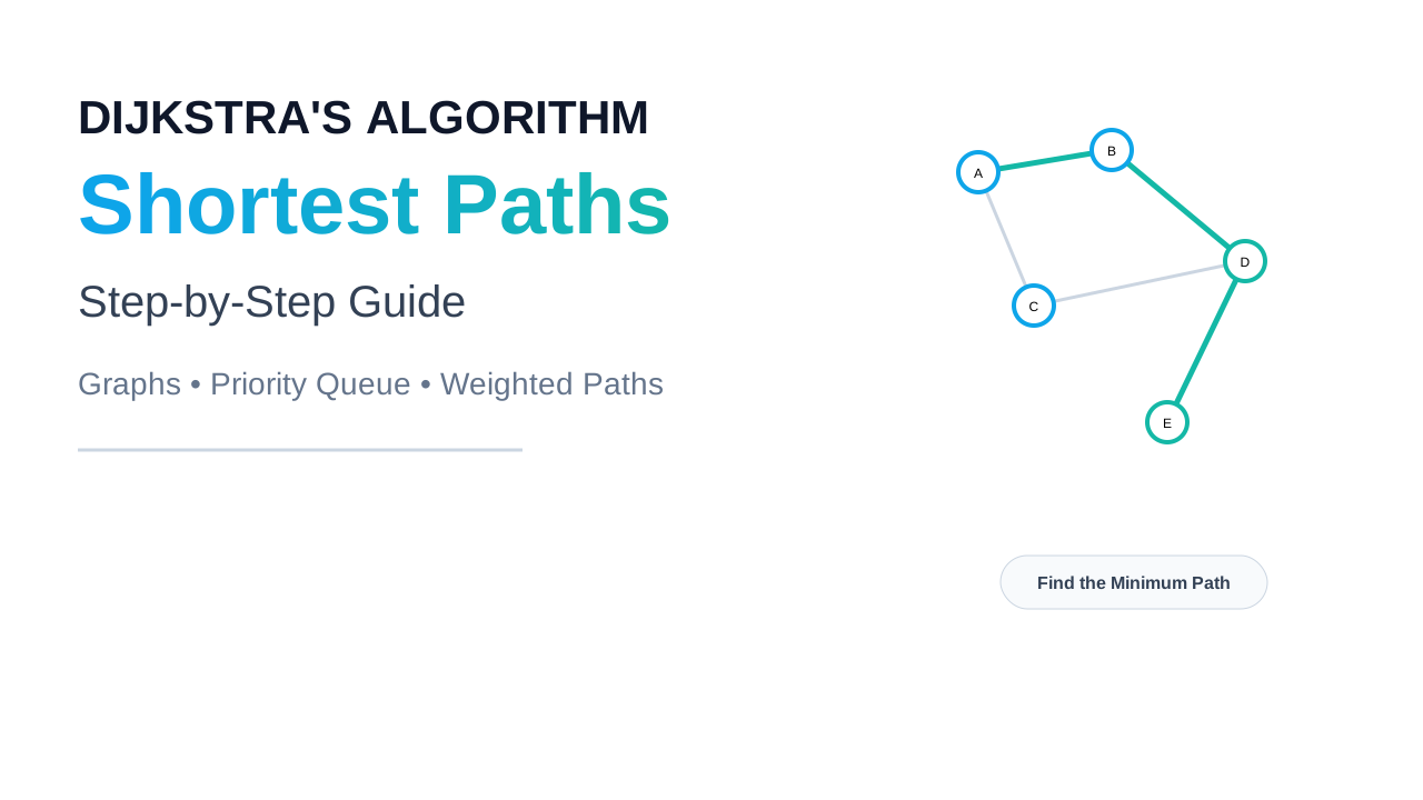
Why Shortest Paths Became a Foundational Problem in Computer Science
Picture a network engineer in the late 1950s trying to route a telephone call across a national switching network. Or picture a logistics planner trying to figure out the cheapest way to move goods between warehouses connected by roads with varying costs, distances, and congestion. In both cases, the underlying structure is the same: a set of points (cities, switches, computers, intersections) connected by paths that each carry some “cost” — distance, latency, price, or time. The question that keeps coming up, over and over, in wildly different domains, is deceptively simple to state and surprisingly hard to answer efficiently: what is the cheapest way to get from A to B?
Before 1956, when Edsger W. Dijkstra devised his now-famous algorithm, the naive way to answer this question was brute force — enumerate every possible path from source to destination, sum up the costs, and pick the minimum. This works fine on paper for a graph with four or five nodes. It becomes catastrophic the moment the graph grows. The number of simple paths between two nodes in a densely connected graph grows combinatorially — it can explode into the billions or more for graphs with just a few dozen nodes. A road network for a mid-sized city has thousands of intersections. A backbone internet topology has tens of thousands of routers. Brute-force path enumeration isn’t just slow on these — it’s computationally infeasible within the lifetime of the universe for large enough inputs.
The real engineering pain point wasn’t just “finding a path” — that’s easy; any depth-first search does that. The pain point was finding the cheapest path efficiently, and doing so without redundant work. Every naive approach that tries to be clever by exploring greedily without any structure ends up either producing wrong answers (because it commits to a locally good choice that turns out to be globally bad) or ends up re-exploring the same territory repeatedly.
This is the problem Dijkstra was solving: how do you systematically, provably, and efficiently discover the shortest path from a single source to every other node in a graph with non-negative edge weights, without wasting computation on paths that can’t possibly be optimal? The answer he arrived at — famously conceived, according to his own recollection, in about twenty minutes while having coffee with his fiancée in Amsterdam — is one of the most reused pieces of algorithmic machinery in computing history. It sits underneath route planning in Google Maps, OSPF and IS-IS routing protocols that keep the internet’s backbone functioning, network latency optimization, robotics motion planning, and — as we’ll get to later — increasingly, the orchestration layers of modern AI agent systems.
Understanding why Dijkstra’s algorithm works, not just how to type it into a text editor, is what separates an engineer who can adapt it to new problems from one who can only copy-paste it.
Building the Mental Model: Greedy Exploration with a Proof of Correctness
Before writing a single line of code, it’s worth building the right intuition, because Dijkstra’s algorithm is one of those algorithms that looks almost too simple once you understand it, and confusingly magical if you don’t.
The graph as a map of costs
Think of a weighted graph as a physical map where every road (edge) has a toll (weight) attached to it, and every intersection (node) is a place you can stand. Your job: starting at node A, figure out the cheapest possible toll cost to reach every other intersection in the map. Crucially, tolls are non-negative — you never get paid to use a road. This constraint turns out to be the linchpin that makes the entire algorithm valid, and we’ll return to why.
The core intuition: expand outward from the cheapest frontier
Imagine standing at the source node with a growing “known territory” — the set of nodes for which you have already determined, with certainty, the shortest possible cost to reach them from the source. Initially, this known territory contains only the source node itself, at cost zero.
At each step, you look at every node on the border of your known territory — nodes that are directly reachable from something already inside your known territory — and you ask: which of these border nodes has the cheapest total cost to reach, given everything you currently know? You pick that node, declare its cost final, and add it to your known territory. Then you look at its outgoing edges and see if they offer cheaper ways to reach other border nodes than what you’d previously recorded.
You repeat this process — expand to the cheapest unexplored frontier node, lock in its distance, relax its neighbors — until every node has been absorbed into the known territory.
Why greedy works here (and why it wouldn’t with negative weights)
This is the part that should click intuitively: because edge weights are never negative, once you pick the frontier node with the smallest tentative distance, there is no possible way a longer, unexplored path could later turn out to be shorter. Any alternative path to that node would have to go through some other frontier node first, and every other frontier node already has a tentative distance greater than or equal to the one you just picked. Adding a non-negative edge weight on top of an already-larger number can never make it smaller. This is precisely why the algorithm breaks with negative weights — a large detour could, in principle, use a negative edge somewhere down the line to become cheaper overall, and Dijkstra’s greedy commitment has no way to see that coming. This is the entire reason algorithms like Bellman-Ford exist as a separate tool for graphs with negative weights.
The priority queue metaphor
If you imagine every border node holding up a numbered sign showing its current best-known cost, the algorithm is simply: repeatedly grab the node holding the smallest sign, finalize it, and then update the signs of its neighbors if you’ve found a cheaper way to reach them. This “always grab the smallest” operation is exactly what a priority queue (typically implemented as a min-heap) is built for, and it’s the data structure that turns this conceptually simple idea into an efficient algorithm.
Internal Working Deep Dive: What Actually Happens Step by Step
This is the heart of understanding Dijkstra’s algorithm — walking through its mechanics precisely enough that you could trace it by hand on paper and predict exactly what a correct implementation should output.
The data structures involved
A working implementation needs four pieces of state:
dist[]— an array or map holding the current best-known shortest distance from the source to every node. Initialized to infinity for every node except the source, which is zero.- A priority queue (min-heap) — holds
(distance, node)pairs, always allowing efficient retrieval of the pair with the smallest distance. visited[]— a boolean array or set tracking which nodes have already been finalized (i.e., are inside the “known territory”).prev[](optional but usually included) — records the predecessor of each node on its shortest path, used later to reconstruct the actual path, not just its cost.
The algorithm’s lifecycle, step by step
Step 1: Initialization. Set dist[source] = 0 and dist[v] = infinity for every other node v. Push (0, source) into the priority queue.
Step 2: Extraction. Pop the pair with the smallest distance from the priority queue. Call this node u with recorded distance d.
Step 3: Staleness check. Because priority queues in most practical implementations don’t support efficient “decrease-key” operations (especially binary heaps in standard libraries like Python’s heapq or Java’s PriorityQueue), it’s common to push a new entry every time a shorter distance is found rather than mutating an existing one. This means the same node can appear multiple times in the queue with different distances. So the first thing to check after popping is: has this node already been finalized, or is this popped distance d larger than the current recorded dist[u]? If so, this is a stale, outdated entry — skip it and move to the next iteration.
Step 4: Finalization. If u is not stale, mark it as visited/finalized. At this point, dist[u] is guaranteed to be the true shortest distance from the source to u — this is the correctness guarantee we built intuition for above, and it never needs to be revisited again.
Step 5: Relaxation. For every neighbor v of u connected by an edge with weight w, compute the candidate distance d + w. If this candidate is smaller than the currently recorded dist[v], this means we’ve just discovered a cheaper way to reach v through u. Update dist[v] = d + w, set prev[v] = u, and push (d + w, v) onto the priority queue.
Step 6: Loop. Repeat from Step 2 until the priority queue is empty (or, in optimized variants, until the specific destination node you care about has been finalized — there’s no reason to keep going once you have the answer you need).
Tracing it by hand
Consider a tiny graph: nodes A, B, C, D. Edges: A→B (4), A→C (1), C→B (2), B→D (1), C→D (5).
- Initialize:
dist = {A:0, B:∞, C:∞, D:∞}. Queue:[(0,A)]. - Pop
(0, A). Finalize A. Relax neighbors: B becomes 4, C becomes 1. Queue:[(1,C), (4,B)]. - Pop
(1, C). Finalize C. Relax neighbors: B via C is1+2=3, which beats the existing 4 — update B to 3. D via C is1+5=6— update D to 6. Queue:[(3,B), (4,B) stale-later, (6,D)]. - Pop
(3, B). Finalize B. Relax neighbors: D via B is3+1=4, which beats existing 6 — update D to 4. Queue:[(4,B) stale, (4,D), (6,D) stale-later]. - Pop
(4, B)— but B is already finalized, so this is stale. Skip. - Pop
(4, D). Finalize D. - Queue empties (remaining stale entries get popped and skipped). Final distances: A=0, B=3, C=1, D=4.
Notice something important here: B’s first discovered distance (4, via direct edge from A) was not the final answer. The algorithm correctly revised it downward to 3 once it discovered the cheaper route through C. This is exactly the “relaxation” mechanism doing its job, and it’s the detail that trips up engineers who assume the first time you touch a node, you’re done with it — you’re not; you’re done with it only once it’s popped and finalized, not merely discovered.
Why finalized nodes never need revisiting
This determinism is the algorithmic payoff of the non-negative weight constraint. Because the priority queue always hands you the globally smallest unfinalized distance, and because you can’t make a distance smaller by adding a non-negative edge weight, there is no future discovery that could ever beat a distance already popped from the top of the heap. This is what allows the algorithm to finalize nodes one at a time, permanently, and never redo work — it’s the source of its efficiency.
Engineering Implementation: From Theory to Production-Quality Code
Now let’s translate the mechanics above into real, runnable code — the kind you’d actually want in a production routing or graph-analytics system, not a toy example that falls apart the moment the graph has more than five nodes.
A clean, idiomatic Python implementation
import heapq
from collections import defaultdict
from typing import Dict, List, Tuple, Optional

class Graph:
    """
    Weighted directed graph represented as an adjacency list.
    Supports non-negative edge weights only — Dijkstra's algorithm
    is not valid for graphs containing negative edge weights.
    """
    def __init__(self):
        self.adjacency: Dict[str, List[Tuple[str, float]]] = defaultdict(list)

    def add_edge(self, u: str, v: str, weight: float, bidirectional: bool = False):
        if weight < 0:
            raise ValueError(
                f"Dijkstra's algorithm requires non-negative weights; "
                f"got {weight} for edge {u}->{v}. Use Bellman-Ford instead."
            )
        self.adjacency[u].append((v, weight))
        if bidirectional:
            self.adjacency[v].append((u, weight))


def dijkstra(
    graph: Graph, source: str, target: Optional[str] = None
) -> Tuple[Dict[str, float], Dict[str, Optional[str]]]:
    """
    Computes shortest distances from `source` to all reachable nodes.
    If `target` is provided, the search can terminate early once the
    target is finalized, saving unnecessary work on large graphs.

    Returns:
        dist: mapping of node -> shortest distance from source
        prev: mapping of node -> predecessor on the shortest path,
              used to reconstruct the actual path later
    """
    dist: Dict[str, float] = defaultdict(lambda: float("inf"))
    prev: Dict[str, Optional[str]] = {}
    dist[source] = 0.0

    # Min-heap of (distance, node). Python's heapq is a binary heap,
    # so we simulate "decrease-key" by pushing duplicate, fresher entries
    # and discarding stale ones on pop -- this is the standard,
    # production-safe pattern for languages without a native decrease-key heap.
    priority_queue: List[Tuple[float, str]] = [(0.0, source)]
    visited: set = set()

    while priority_queue:
        current_dist, u = heapq.heappop(priority_queue)

        if u in visited:
            continue  # stale entry, already finalized with a better distance
        visited.add(u)

        if target is not None and u == target:
            break  # early exit once the node we actually care about is finalized

        for neighbor, weight in graph.adjacency[u]:
            if neighbor in visited:
                continue
            candidate = current_dist + weight
            if candidate < dist[neighbor]:
                dist[neighbor] = candidate
                prev[neighbor] = u
                heapq.heappush(priority_queue, (candidate, neighbor))

    return dict(dist), prev


def reconstruct_path(prev: Dict[str, Optional[str]], source: str, target: str) -> List[str]:
    """Walks the prev[] chain backward from target to source."""
    path = [target]
    node = target
    while node != source:
        node = prev.get(node)
        if node is None:
            return []  # target unreachable from source
        path.append(node)
    path.reverse()
    return path


if __name__ == "__main__":
    g = Graph()
    g.add_edge("A", "B", 4)
    g.add_edge("A", "C", 1)
    g.add_edge("C", "B", 2)
    g.add_edge("B", "D", 1)
    g.add_edge("C", "D", 5)

    distances, predecessors = dijkstra(g, "A")
    print("Shortest distances from A:", distances)
    print("Shortest path A -> D:", reconstruct_path(predecessors, "A", "D"))
Design decisions worth calling out explicitly
Why a min-heap and not a sorted list. A naive implementation might maintain a sorted list of (distance, node) pairs and always pull the front. Insertions into a sorted list cost O(n) in the worst case because you have to shift elements. A binary heap gives you O(log n) insertion and O(log n) extraction, which is the difference between an algorithm that scales to graphs with millions of nodes and one that grinds to a halt past a few thousand.
Why we tolerate duplicate/stale queue entries instead of decrease-key. Some textbook presentations of Dijkstra’s algorithm assume access to a priority queue with an efficient decrease-key operation, achieving the theoretically optimal O(E + V log V) complexity using structures like Fibonacci heaps. In practice, almost no mainstream standard library (Python, Java, C++’s std::priority_queue, Go’s container/heap) exposes an efficient decrease-key primitive out of the box. The pragmatic, widely-used engineering solution — pushing a new entry every time a shorter distance is found, and simply discarding stale pops — is simpler to implement correctly, avoids a whole class of heap-corruption bugs, and only costs a modest constant-factor overhead in practice. This trade-off between theoretical optimality and implementation robustness is a recurring theme in real systems engineering, and it’s worth understanding rather than memorizing.
Why early termination matters for target-specific queries. If you only care about the shortest path to one specific destination — the overwhelmingly common case in a routing application like “give me directions from my house to the airport” — there is no reason to keep running the algorithm until every node in the entire graph is finalized. The moment the target node is popped and finalized, you have your answer, and everything else is wasted computation. On a graph the size of a national road network, this optimization alone can be the difference between milliseconds and seconds of latency.
Validating non-negative weights at the data layer. Rather than letting negative weights silently produce wrong answers deep inside the algorithm (which is a brutal class of bug to trace), the add_edge method above rejects them immediately with a clear error pointing the engineer toward Bellman-Ford. Defensive validation at the boundary of a system is cheap insurance against a much more expensive debugging session later.
Complexity analysis
With a binary heap, each node is popped once (O(V) pops) and each edge triggers at most one push (O(E) pushes), and each heap operation costs O(log V). This gives an overall time complexity of O((V + E) log V), which simplifies to O(E log V) for connected graphs where E ≥ V − 1. Space complexity is O(V + E) for the graph representation plus O(V) for the distance and heap bookkeeping. For sparse graphs — the common case in road networks and most real-world graphs, where the number of edges is roughly linear in the number of nodes rather than quadratic — this is extremely efficient and comfortably handles graphs with millions of nodes in production systems.
Common implementation mistakes
A recurring bug is forgetting the staleness check and re-processing a node’s neighbors every time any entry for that node is popped, not just the first (correct) one — this doesn’t produce wrong answers, but it silently destroys the algorithm’s efficiency guarantees by redoing enormous amounts of redundant relaxation work. Another common mistake is running Dijkstra’s algorithm on a graph that secretly contains a negative-weight edge (for example, representing a discount or rebate as a negative cost) — the algorithm won’t crash, it will simply produce a wrong answer with total confidence, which is far more dangerous than an outright failure. A third mistake, especially in interview settings, is confusing the “discovered” distance (the first time you find any path to a node) with the “finalized” distance (the shortest path, guaranteed) — code that returns as soon as a node is first reached, rather than waiting until it’s popped from the top of the heap, is simply incorrect.
Real-World Systems: How the Industry Actually Uses This
Network routing protocols
Link-state routing protocols like OSPF (Open Shortest Path First) and IS-IS, which form the backbone of how large corporate and internet-service-provider networks compute routing tables, run a variant of Dijkstra’s algorithm directly on their internal graph representation of the network topology, where edge weights represent link cost (often derived from bandwidth). Every router periodically recomputes its shortest-path tree to every other router in the area, which is precisely a single-source-shortest-path Dijkstra run.
Mapping and logistics
Modern routing engines like those behind Google Maps or logistics companies’ delivery-route optimizers don’t run textbook Dijkstra directly at planetary scale — the graph of every road segment on Earth is far too large for a naive single run to be fast enough for an interactive user experience. Instead, they build on top of Dijkstra’s core idea with heavy optimizations: A* search, which augments Dijkstra with a heuristic (like straight-line distance to the destination) to bias exploration toward the goal and dramatically prune the search space; contraction hierarchies, which precompute shortcut edges through “unimportant” intersections so that long-distance queries can skip over vast swaths of local road detail; and bidirectional search, which runs Dijkstra simultaneously from both the source and the destination and stops when the two frontiers meet. Every one of these production techniques is a layer on top of Dijkstra’s core correctness guarantee, not a replacement for it — understanding vanilla Dijkstra is the prerequisite for understanding why these optimizations are valid.
Cloud infrastructure and distributed systems
Within large cloud providers, shortest-path-style algorithms show up in unexpected places: optimizing data placement and replication paths to minimize latency across data center topologies, computing least-cost paths through software-defined networking (SDN) control planes, and load-balancing traffic across a mesh of microservices where “cost” might represent latency or current load rather than physical distance.
AI Era Relevance: Why This Still Matters in 2026
It would be easy to assume that a 1959-era algorithm has little to say to the world of large language models and autonomous agents — but the opposite is increasingly true, precisely because AI systems in 2026 are built as graphs of components, and graph problems keep resurfacing wherever there’s a graph.
Agentic workflow orchestration. Modern AI agent frameworks represent a task as a graph of possible tool calls, sub-agent invocations, or reasoning steps, where each edge might carry an associated cost — latency, API price, or token consumption. When an orchestration layer needs to decide the cheapest sequence of tool calls to accomplish a goal, that’s structurally a shortest-path problem, and Dijkstra-style greedy frontier expansion is a natural fit whenever the “cost” of each step is known and non-negative.
Retrieval-Augmented Generation (RAG) and knowledge graphs. Many production RAG systems that go beyond flat vector search build a knowledge graph of entities and relationships. Answering “what connects concept A to concept C” or finding the most relevant chain of relationships between two entities is a shortest-path query over that knowledge graph, sometimes weighted by embedding-similarity distance rather than physical cost.
Multi-agent systems and task routing. In multi-agent architectures, deciding which chain of specialized agents should handle a request — where each hand-off has an associated latency or cost — is again a shortest-path problem over a graph of agent capabilities. As agentic systems scale into meshes of dozens or hundreds of specialized agents, the naive “try everything” approach becomes exactly the same brute-force trap that motivated Dijkstra in the first place, and the same greedy-frontier discipline becomes relevant again.
ML infrastructure and model routing. Systems that route a given inference request across a fleet of models or GPU clusters based on latency, cost, and load are, at their core, solving weighted shortest-path or min-cost-flow problems, of which Dijkstra’s algorithm is a foundational building block.
The throughline is that AI engineering in 2026 is not just about training and prompting models — it’s increasingly about building efficient systems around models, and systems are graphs. The classical algorithms that solve graph problems efficiently don’t become obsolete; they become the plumbing.
Advantages, Limitations, and Trade-offs
Advantage: guaranteed correctness with non-negative weights. Dijkstra’s algorithm doesn’t just find a short path — it provably finds the shortest one, with a clean mathematical argument backing it up. This matters enormously in systems where being wrong isn’t a minor inconvenience — a mis-routed network packet, an under-priced logistics quote, or an incorrect agent-orchestration cost estimate can have real downstream costs.
Advantage: efficient enough for genuinely large graphs. With a binary heap, O(E log V) complexity is fast enough to handle graphs with millions of edges within a reasonable time budget, which is why it remains the default choice rather than a historical curiosity.
Limitation: breaks down with negative edge weights. This is the algorithm’s most important boundary. The moment a graph can contain a negative-weight edge — representing something like a rebate, a discount, or a “help me undo prior cost” scenario — Dijkstra’s greedy finalization can produce confidently wrong answers, because a not-yet-explored path might later turn out to be cheaper thanks to a negative edge deep inside it. In these situations, engineers reach for Bellman-Ford, which tolerates negative weights (though not negative cycles) at the cost of higher time complexity, O(V·E).
Limitation: single-source, not naturally all-pairs. Dijkstra’s algorithm computes shortest paths from one source to every other node. If you need shortest paths between every pair of nodes in a dense graph, running Dijkstra V times (once per source) costs O(V·E log V), and at that scale it’s often more efficient to switch to the Floyd-Warshall algorithm, which computes all-pairs shortest paths directly in O(V³) — a better trade depending on graph density.
Trade-off: memory versus recomputation. Storing the full prev[] predecessor map for path reconstruction costs additional memory proportional to the number of nodes; in memory-constrained embedded or edge-computing contexts, engineers sometimes choose to recompute paths on demand rather than store them, trading CPU cycles for memory footprint.
Trade-off: exactness versus speed at planetary scale. As discussed above, production mapping systems don’t run raw Dijkstra at the scale of “every road on Earth” because even O(E log V) becomes too slow for an interactive user waiting on a response. They accept the engineering complexity of precomputed contraction hierarchies and heuristic-guided A* search in exchange for millisecond-level query times — a clear illustration that “the theoretically correct algorithm” and “the production-ready system” are not always the same artifact, even when the former is the conceptual foundation of the latter.
Career Impact and What to Learn Next
Dijkstra’s algorithm remains one of the most consistently asked topics in technical interviews at every tier of the industry — not because interviewers expect candidates to have memorized the code verbatim, but because it’s an excellent lens for testing whether a candidate genuinely understands greedy algorithms, priority queues, and graph traversal, or has only memorized surface patterns. Being able to explain why it fails with negative weights, and what you’d reach for instead, is often a stronger signal to an interviewer than reciting the implementation flawlessly.
Beyond interviews, fluency with shortest-path algorithms is directly relevant to roles in backend infrastructure engineering, network engineering, logistics and supply-chain systems, mapping and geospatial platforms, distributed-systems and platform engineering, and increasingly, AI infrastructure and agent-orchestration engineering — any role where you’re building systems on top of graphs with associated costs.
If this topic clicked for you, the natural next steps are: study A* search to see how a heuristic function accelerates Dijkstra toward a specific goal; study Bellman-Ford to understand how negative weights are handled and how negative cycles are detected; study Floyd-Warshall for the all-pairs case; and study min-cost max-flow algorithms, which extend these same greedy-and-relax ideas into problems involving both cost and capacity constraints — a common pattern in resource-allocation systems, including modern GPU-scheduling and inference-routing infrastructure.
Conclusion
Dijkstra’s algorithm endures not because it’s the flashiest technique in computer science, but because it solves a problem that never actually goes away: given a network of costs, how do you make the provably cheapest decision without wasting effort exploring paths that can’t possibly win? That question was just as urgent for a 1959 telephone network as it is for a 2026 fleet of AI agents deciding which chain of tool calls minimizes latency and token spend. The specific graphs keep changing — roads, routers, knowledge graphs, agent meshes — but the underlying discipline of greedy, provably-correct frontier expansion keeps resurfacing, because it is, in a very real sense, one of the cleanest expressions of “do the locally optimal thing, and prove that it stays globally optimal” that computer science has ever produced. Understanding it deeply — not just being able to type it, but being able to explain why it works, where it breaks, and what you’d reach for instead — is a durable piece of engineering judgment that will keep paying off long after the specific syntax of any given programming language has been forgotten.